Contingency Tables Part I: The Potential Outcomes Framework
(This is the first post in a planned series about the design and analysis of A/B tests. Subscribe to my newsletter at the bottom to be notified about future posts.)
Imagine we have run an A/B test like the one illustrated in Figure 1. A thousand people are exposed to some legacy experience, and one hundred of those people do something good, e.g. they buy something. Another thousand people see some new thing, and one hundred and thirty buy something. We can summarize these results in a contingency table which makes it easy to compare the two groups, and is especially helpful for analysis. But what do we need to analyze? It certainly seems like the new thing is better than the old thing! After all, you don’t need a PhD in statistics to know that 130 > 100.
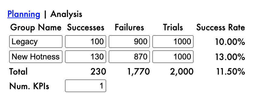
Figure 1: A contingency table (from my <a href='https://abtesting.convexanalytics.com'>A/B testing calculator</a>).
I think there’s this resentment that sometimes builds up between data scientists and non-data scientists when looking at results like this. As if non-data scientists need permission to conclude that 130 > 100, and statistical significance is what gives them that permission. As if data scientists were some sort of statistics mafia who need to be “consulted” if you know what’s good for you.
I can assure you, 130 is greater than 100, and statistical significance doesn’t have anything to do with it. The problem is, this is the wrong comparison.
Figure 2: A hilarious internet meme.
There were 2000 people in this test. What do we think would have happened if we had shown all of them the legacy experience? Of course, we can only speculate about this, because that’s not what happened. If the results of this A/B test are a reasonable proxy, we might think that around 10% of them (around 200) would have purchased. But it would be silly to pretend we know exactly what would have happened in that scenario. Nobody can do a perfect job of speculating.
What do we think would have happened if all 2000 had experienced the new thing? Again, we don’t know—we can’t know—exactly, but it seems reasonable to speculate that around 13% of them (around 260) would have purchased.
There are a lot of weasel words in the last two paragraphs, and that’s because we are speculating about two situations, neither of which actually happened. It’s like, a person can speculate about what would have happened if Hillary had won the election in 2016, or if Bernie had won the nomination that year. But anyone who says they know exactly what would have happened is mistaken.
Nevertheless, this is the comparison we actually care about: comparing the outcome where everyone had the legacy experience with the outcome where everyone has the new experience. Neither of these things actually happened, but this is the comparison we actually care about. And this is the problem that statistics tries to solve: the comparison we care about, we can’t make; and the comparison we can make, we don’t care about!
In causal inference, the two scenarios we care about are called potential outcomes, and comparing potential outcomes is essential for smart decision making. But it’s easy to see that we can only ever observe at most one of the potential outcomes. If we decide to show the new experience to everyone, we give up any hope of learning what would have happened had we shown the old experience to everyone. An A/B test is a hybrid: we give up on observing either of the potential outcomes, but in exchange we get some insight into what both potential outcomes might look like.
Here’s another complication: what if this A/B test isn’t a good proxy for what would have happened in those hypothetical situations? What if the sorts of people in the first group are just completely different than the sorts of people in the second group? Like let’s say it’s an ad for a remote control car, and the only people in the first group are people who hate fun, and the only people in the second group are children and engineers with disposable income? The fact that fewer people in the first group purchased says more about those people and less about the ad that was shown.
That’s why it is so important to verify “covariate balance”: checking that relevant demographical and behavioral patterns are comparable in the two groups. When we randomly assign people to groups, the law of large numbers guarantees all covariates will be approximately balanced, but because it’s random we can get some fluctuations. It’s always a good idea to check, and if there is a (small) imbalance, we can correct for it after the fact. Even better, if there are some factors we think are especially important to balance, like gender or economic status, we can use a process called stratification to make sure they’re balanced when we design the test.
Another problem that can arise is interaction between the two groups. For example, let’s say the first group doesn’t see an ad at all, and the second group does. Let’s say Alice is in the first group and Brian is in the second. Neither of them buy the remote control car. But had Alice seen the ad, not only would she have bought the car, she would have called her friend Brian and persuaded him to buy one too so they can race! In this scenario, what Brian does depends on what Alice experiences.
Humans being social creatures, it’s easy to imagine this happens pretty frequently, and researchers bend over backwards to avoid it. There just isn’t a great way of taking it into account. Instead, researchers try to separate people so that what one person experiences does not influence what another person does. This assumption is called the “stable unit treatment value assumption” or SUTVA, which is one of those terms that doesn’t begin to describe what it actually means, but is nonetheless an essential assumption in causal inference. (I wrote more about SUTVA here.)
Even when the covariates are balanced and SUTVA holds, because people are randomly assigned to groups, the observed results are still not a perfect proxy for what would have happened in the two scenarios we care about. Is a number that’s around 260 greater than a number that’s around 200? Yeah, probably, depending on what we mean by “around” and “probably”. Again, these are weasel words, and we need statistics to explain exactly what we know and don’t know about the two hypothetical scenarios we’re trying to compare.
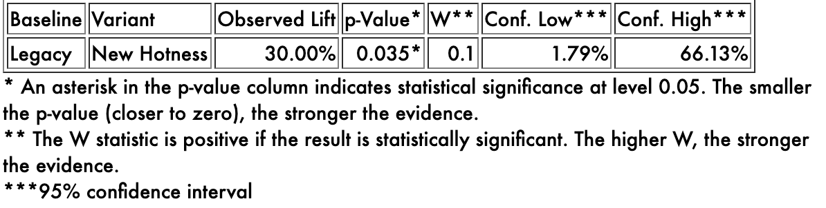
Figure 3: A confidence interval (from my <a href='https://abtesting.convexanalytics.com'>A/B testing calculator</a>).
Without a doubt, 130 > 100, but do we think that a number around 260 is greater than a number around 200? How much bigger? The p-value answers the first question: the lower the p-value, the more confident we are that the observed comparison is at least directionally correct. The smaller the p-value, the more confident we are that a number around 260 is in fact greater than a number around 200, even though we don’t know exactly what those two numbers are. How confident is confident enough? That depends on context, like whether someone’s life is at stake, but typically if the p-value is less than 0.05, we say the result is statistically significant, and that threshold defines what is “confident enough”.
(The proper interpretation of p-values is quite challenging because of the multiple comparisons problem. I created a number called the W statistic specifically for this reason. I could—and eventually will—fill an entire other post on this topic.)
The confidence interval answers the “how much bigger” question. Some numbers around 260 are quite a bit higher than some other numbers around 200. Some numbers around 260 are only slightly higher than some other numbers around 200. Even though this particular result is statistically significant, all that tells us is we think the new experience is in fact better than the old one. It could be slightly better, or way better, or anywhere in between.
The confidence interval gives us a plausible range of values that are consistent with what we have observed. In this case, there is quite a bit of uncertainty! Even though we observed the new experience to be 30% better than the legacy, that is only true for a haphazardly chosen half of the audience! We don’t know exactly how much better the new experience would have been, had we shown it to everyone, compared to the legacy experience, had we shown it to everyone, because neither of those things actually happened. But we can be reasonably confident that it would have been at least 1.79% better. And we can be confident that it wouldn’t have been more than 66.13% better. And yeah, it probably would have been around 30% better. But we just can’t know for sure, because that comparison we actually care about isn’t what actually happened.
So that’s why data scientists care about sample sizes, and p-values, and confidence intervals. Because we’re trying to compare two hypothetical scenarios which by definition cannot both actually occur. Instead, we create a situation in which neither of these scenarios occur, so that we can learn about both of them. It actually works pretty well! In fact, it works better than literally anything else the human race has ever come up with. But it still doesn’t work perfectly, and that’s why if you look at a test like this and conclude that 130 > 100, your data scientist friend is going to die a little inside.
Like this post? Check out the next in the series here.