Viterbi Algorithm, Part 1: Likelihood

The Viterbi algorithm is used to find the most likely sequence of states given a sequence of observations emitted by those states and some details of transition and emission probabilities. It has applications in Natural Language Processing like part-of-speech tagging, in error correction codes, and more!

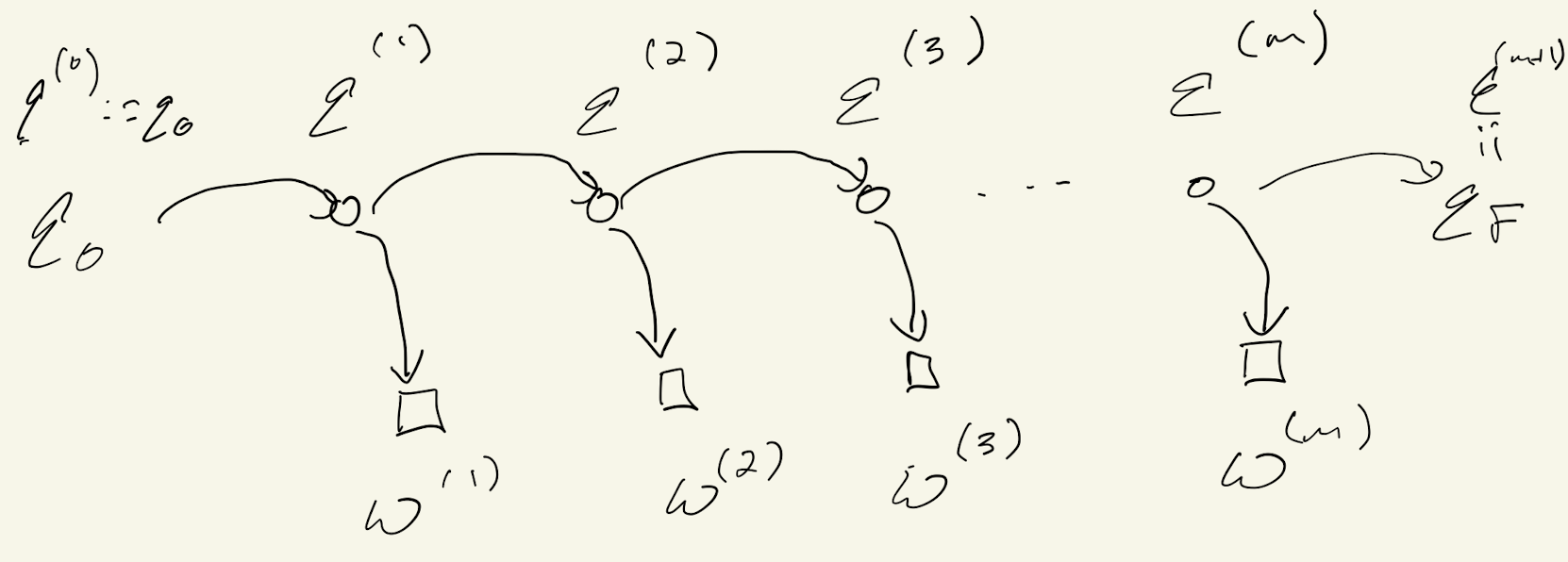
Our presentation follows Jurafsky and Martin closely, merely filling in some details omitted in the text. Regardless of the application, we formulate the problem as a Hidden Markov Model as illustrated in Figure 1. What we observe is a sequence of words or symbols $w^{(1)}, w^{(2)}, \ldots, w^{(m)}.$ These words are assumed to belong to a vocabulary $V = \{ w_1, w_2, \ldots, w_{|V|} \}.$

Corresponding to these observations are a sequence of states $q^{(1)}, \ldots, q^{(m)}.$ The states are assumed to belong to a set $Q =\{q_1, \ldots, q_N \}.$ In addition, there are two special states, $q_0$ and $q_F,$ representing the beginning and end of the sequence. For convenience, we will use $w_i^j$ to denote the word sequence $w^{(i)} \cdots w^{(j)}$ and $q_i^j$ to denote the state sequence $q^{(i)} \cdots q^{(j)}.$

A Hidden Markov Model (HMM) is characterized by a set of transition probabilities $A$ and a set of emission probabilities $B.$ The transition probabilities include $a_{ij},$ the probability of transitioning from state $q_i$ to $q_j;$ $a_{0j},$ the probability of transitioning from $q_0$ to $q_j;$ and $a_{iF},$ the probability of transitioning from $q_i$ to $q_F.$ The emission probabilities are denoted $b_i(w_k),$ the probability of emitting word $w_k$ from state $q_i.$ In what follows, when we say “given the HMM”, what we mean is “given the transition and emission probabilities”.

Jurafsky and Martin describe three problems we may wish to solve associated with this context. First, characterizing the likelihood of a word sequence given the HMM. Second, finding the most likely state sequence $q_1^m$ given the word sequence $w_1^m$ and the HMM. This is called decoding. Finally, learning the HMM (that is, $A$ and $B$) based on one or more observed sequences of words and states. (Notably, Jurafsky and Martin’s formulation assumes a single, presumably long sequence. I think it is more interesting to permit multiple, possibly short sequences.)

Likelihood

In this section, we derive an algorithm, called the Forward Algorithm, for solving the likelihood problem: calculating $P\{w_1^m \; | \; A, B \}.$ Again, our derivation follows Jurafsky and Martin closely, but with more details filled in.

We will make the following assumptions:

• Word Independence: $P\{ w_1^m \; | \; q_1^m \} = \Pi_{t=1}^m P\{ w^{(t)} \; | \; q^{(t)} \}.$ This assumption is two-fold: it says first that words $w^{(i)}$ and $w^{(j)}$ are conditionally independent given $q_1^m,$ and second that $w^{(t)}$ is conditionally independent of $q^{(i)}$ given $q^{(t)},$ $i \neq t.$
• Markov Assumption: $P\{ q_1^m \; | \; A, B \} = \Pi_{t=1}^m P \{ q^{(t)} \; | \; q^{(t-1)} \}.$ This says that a state is conditionally independent of earlier states given the preceding state.
• Known Transition and Emission Probabilities: the notation makes it clear, but it’s worth emphasizing that in this section we will assume the HMM is known. In practice this would not be the case! The learning problem mentioned above and to be described later addresses this.

Applying the Law of Total Probability followed by the definition of conditional probability, we have $$ \begin{align} P\{w_1^m \; | \; A, B \} &= \sum_{q_1^m} P\{w_1^m, q_1^m \; | \; A, B \} \\ &= \sum_{q_1^m} P\{w_1^m \; | \; q_1^m, A, B \} \cdot P\{q_1^m \; | \; A, B \} \end{align} $$

Applying Word Independence and the Markov Assumption allows us to calculate each term in the sum easily enough, but the sum is over all $N^m$ possible state sequences. So the naive solution has runtime at least $\mathcal{O}(N^m).$ The Forward Algorithm is a clever approach for avoiding calculating these sums. The central quantity is $$ \alpha_t(j) := P \{ w_1^t, q^{(t)} = q_j \; | \; A, B \}, $$ which in words is the joint probability of the word sequence through word $t$ and that the $t$th state is $q_j.$ To motivate this quantity, note that $$ \begin{align} P\{w_1^m \; | \; A, B \} &= \sum_{q_j} P \{ w_1^m, q^{(m)} = q_j \; | \; A, B \} \\ &= \sum_j \alpha_m(j). \end{align} $$

Calculating $\alpha_1(j)$ is straightforward enough: $$ \begin{align} \alpha_1(j) &= P \{ w^{(1)}, q^{(1)} = q_j \; | \; A, B \} \\ &= P \{ w^{(1)} \; | \; q^{(1)} = q_j, A, B \} \cdot P \{ q^{(1)} = q_j \; | \; A, B \} \\ &= b_j \left( w^{(1)} \right) \cdot a_{0j}. \end{align} $$

For $t > 1,$

$$ \begin{align} \alpha_t(j) &= \sum_{i=1}^N P \{ w_1^t, q^{(t-1)} = q_i, q^{(t)} = q_j \; | \; A, B \} \\ &= \sum_{i=1}^N P\{ w^{(t)} \; | \; w_1^{t-1}, q^{(t-1)} = q_i, q^{(t)} = q_j, A, B \} \\ &\phantom{=} \hspace{30pt} \cdot P \{ w_1^{t-1}, q^{(t-1)} = q_i, q^{(t)} = q_j \; | \; A, B \}, \end{align} $$ where the first line follows from the Law of Total Probability and the second from the definition of conditional probability. Next we apply the Word Independence assumption and the definition of the emission probabilities to simplify: $$ \begin{align} \alpha_t(j) &= \sum_{i=1}^N P\{ w^{(t)} \; | \; w_1^{t-1}, q^{(t-1)} = q_i, q^{(t)} = q_j, A, B \} \\ &\phantom{=} \hspace{30pt} \cdot P \{ w_1^{t-1}, q^{(t-1)} = q_i, q^{(t)} = q_j \; | \; A, B \} \\ &= \sum_{i=1}^N P\{ w^{(t)} \; | \; q^{(t)} = q_j, A, B \} \\ &\phantom{=} \hspace{30pt} \cdot P \{ w_1^{t-1}, q^{(t-1)} = q_i, q^{(t)} = q_j \; | \; A, B \} \\ &= \sum_{i=1}^N b_j \left( w^{(t)} \right) \cdot P \{ w_1^{t-1}, q^{(t-1)} = q_i, q^{(t)} = q_j \; | \; A, B \}. \end{align} $$

Next, we expand the term on the right using the definition of conditional probability, and apply our Word Independence assumption again: $$ \begin{align} \alpha_t(j) &= \sum_{i=1}^N b_j \left( w^{(t)} \right) \cdot P \{ w_1^{t-1}, q^{(t-1)} = q_i, q^{(t)} = q_j \; | \; A, B \} \\ &= \sum_{i=1}^N b_j \left( w^{(t)} \right) \cdot P \{q^{(t)} = q_j \; | \; w_1^{t-1}, q^{(t-1)} = q_i, A, B \} \\ &\phantom{=} \hspace{30pt} \cdot P \{ w_1^{t-1}, q^{(t-1)} = q_i \; | \; A, B \} \\ &= \sum_{i=1}^N b_j \left( w^{(t)} \right) \cdot P \{q^{(t)} = q_j \; | \; q^{(t-1)} = q_i, A, B \} \\ &\phantom{=} \hspace{30pt} \cdot P \{ w_1^{t-1}, q^{(t-1)} = q_i \; | \; A, B \} \\ &= \sum_{i=1}^N b_j \left( w^{(t)} \right) \cdot a_{ij} \cdot \alpha_{t-1}(i), \end{align} $$ with the last line following from the definition of the transition probabilities, and from the definition of $\alpha_{t-1}(i),$ respectively.

The following python code illustrates how to calculate the quantities we need:

def forward_algorithm(w1m, a, a0, b):
    """
    Parameters
    ----------
     w1m : list of length m
         Sequence of word indices; wlm[t] is the index of the t-th word
     a : N x N array
         State transition probabilities
     a0 : N x 1 array
         Initial transition probabilities
     b : N x |V| array
         Word emission probabilities

    Returns
    -------
     P_w1m : float
         P{w1m | A, B}
    """
    N = len(a0)
    m = len(w1m)
    alpha = np.zeros(m, N)
    for j in range(N):
        alpha[0, j] = b[j, w1m[0]] * a0[j]

    for t in range(1, m):
        for j in range(N):
            for i in range(N):
                alpha[t, j] += alpha[t-1, i] * a[i, j] * b[j, wlm[t]]

    P_w1m = 0
    for j in range(N):
        P_wlm += alpha[m-1, j]

    return P_w1m

Based on the three nested for loops, the runtime of this algorithm is plainly $\mathcal{O}(N^2 m),$ much better than the naive algorithm.